This post will cover how a researcher can efficiently extract variables from Medicare Cost Reports and create a usable dataset for either cross-sectional or panel analysis. It demonstrates the use of the medicare R package, which was written and published by Health Policy Data Analyst Robert Gambrel. While the NBER publishes cleaned datasets of select variables, a researcher will have to know how to handle the raw datasets in order to extract variables of interest that aren’t available there.
Cost Reports: Background
CMS publishes Cost Report data for Hospitals and Post Acute Services as well as Hospices. Unfortunately, these raw datasets are in long format; each “row” of the raw datasets have 5 columns: a report number, a worksheet number, a row number, a column number, and an item value. In order to extract variables of interest, a researcher must review the actual workbooks that providers complete and determine which worksheet, row, and column are needed to subset to get the item value of interest. Entries can then be merged based on the report number.
In my experience, the appropriate documentation files are:
- Chapter 32: Home Health Agencies
- Chapter 35: Skilled Nursing Facilities
- Chapter 36: Hospitals
- Chapter 38: Hospices
Hospices and HHA’s have used the same reporting forms since the mid 1990’s. Skilled nursing facilities and hospitals, however, switched their reporting guidelines in 2010. Therefore, writing extracts for variables from the 1996 forms will not work for data from the 2010 form. Crosswalks are available in the documentation files linked on the sidebar here. Once you find the variable you want in the 1996 form, it’s easy to translate the worksheet number, row, and column to the newer format. It’s good practice to check a few facilities’ results from both sources to make sure that the data is consistent across the reporting switch; this will ensure your extracts are working for both periods.
Hospice Cost Reports Demonstration
We’ll start by downloading and extracting the hospice cost report data.
Hospice data is smaller than data from other sources, doesn’t change
reporting systems in 2010, and is available all in one download.
Download
it
(by clicking Hospice Data files). Also, download the documentation
file for hospices linked above.
We’ll start with the 2014 data.
library(medicare)
library(dplyr)
library(magrittr)
library(readr)
# optional for final maps
library(ggplot2)
library(maps)

alpha_14 <- read_csv("~/Downloads/HOSPC-ALL-YEARS/hospc_2014_alpha.csv", col_names = F)
nmrc_14 <- read_csv("~/Downloads/HOSPC-ALL-YEARS/hospc_2014_nmrc.csv", col_names = F)
rpt_14 <- read_csv("~/Downloads/HOSPC-ALL-YEARS/hospc_2014_rpt.csv", col_names = F)
These are pretty uninterpretable at first glance, and they don’t have variable names by default. Those are all available in the documentation, but I’ve made a wrapper to make it quick and painless to name. Still, it’s hard to know what to make of the data.
names(alpha_14) <- medicare::cr_alpha_names()
names(nmrc_14) <- cr_nmrc_names()
names(rpt_14) <- cr_rpt_names()

lapply(list(alpha_14, nmrc_14, rpt_14), head)

## [[1]]
## # A tibble: 6 × 5
##   rpt_rec_num wksht_cd line_num clmn_num
##         <int>    <chr>    <chr>    <chr>
## 1       34033  A000000    00100     0000
## 2       34033  A000000    00200     0000
## 3       34033  A000000    00300     0000
## 4       34033  A000000    00400     0000
## 5       34033  A000000    00500     0000
## 6       34033  A000000    00600     0000
## # ... with 1 more variables: itm_alphanmrc_itm_txt <chr>
##
## [[2]]
## # A tibble: 6 × 5
##   rpt_rec_num wksht_cd line_num clmn_num itm_val_num
##         <int>    <chr>    <chr>    <chr>       <int>
## 1       34033  A000000    00400     0300          52
## 2       34033  A000000    00400     0600          52
## 3       34033  A000000    00400     0800          52
## 4       34033  A000000    00400     1000          52
## 5       34033  A000000    00500     0500           1
## 6       34033  A000000    00500     0600           1
##
## [[3]]
## # A tibble: 6 × 18
##   rpt_rec_num prvdr_ctrl_type_cd prvdr_num   npi rpt_stus_cd  fy_bgn_dt
##         <int>              <int>     <chr> <chr>       <int>      <chr>
## 1       34033                  4    111714  <NA>           1 11/26/2013
## 2       34071                  4    341598  <NA>           1 10/23/2013
## 3       34375                  5    031621  <NA>           1 10/11/2013
## 4       35065                  4    361664  <NA>           1 10/01/2013
## 5       35167                  6    671777  <NA>           1 11/01/2013
## 6       35451                  5    671784  <NA>           1 11/11/2013
## # ... with 12 more variables: fy_end_dt <chr>, proc_dt <chr>,
## #   initl_rpt_sw <chr>, last_rpt_sw <chr>, trnsmtl_num <chr>,
## #   fi_num <chr>, adr_vndr_cd <chr>, fi_creat_dt <chr>, util_cd <chr>,
## #   npr_dt <chr>, spec_ind <chr>, fi_rcpt_dt <chr>
You’d be correct in surmising that rpt_rec_num is the internal link
between the three files. The rpt file has one entry per hospice
submission (usually just one per year, but sometimes more). The alpha
and nmrc files, though, have many. They do this because they have to
collapse data from multiple spreadsheets into one uniform format. Each
row points to a cell on a given worksheet.
ALPHA and NMRC data
To subset a variable, you’ll need to look through the actual worksheets that facilities fill out. If you download the documentation linked above for hospice, you’ll find an Excel spreadsheet file with multiple pages (under R9P238f, open R9P238f.xls). Some sheets have address and location info. Others report patient counts and treatment days. Still others have staffing information and revenue / cost annual totals. Here is an example of one worksheet page (among many!):
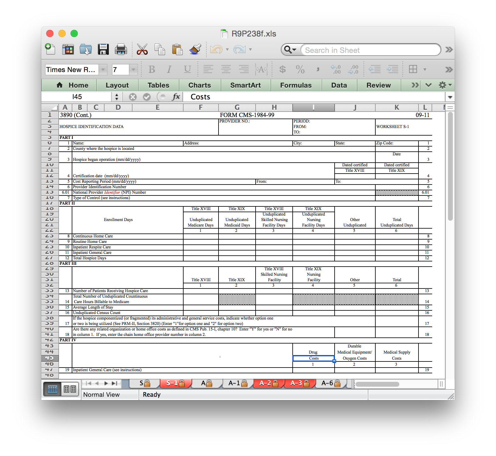
First, we can see that the hospice name is on worksheet S-1. Lines are numbered, and it’s on row 1; similar for columns, we can see that it’s in column 1. Note that column numbers are conditional on how the row is laid out and not absolute references to Excel column numbers; the first column with information in line 1 is not the same absolute Excel column as the first column with patient information on line 8.
The file convention is that the worksheet is always 6 characters, with
no punctuation, with trailing 0’s. Rows and columns are always
multiplied by 100. Since the name is an alphanumeric value, we should
expect to find it in the alpha file. Note what happens if we try to
extract it from the nmrc file.
hospice_names <- medicare::cr_extract(alpha_14, "S100000", 100, 100, "hospice_name")
nrow(hospice_names)

## [1] 2818

hospice_names_nmrc <- cr_extract(nmrc_14, "S100000", 100, 100, "hospice_name")

## Warning in subset_row(worksheet_subset, row): No data found with specified
## row number.

## Warning in subset_column(row_subset, column): No data found with specified
## column number.

## Warning in cr_extract(nmrc_14, "S100000", 100, 100, "hospice_name"): Final
## result has no data. Double-check parameters or consider switching alpha/
## nmrc extraction dataset.
Several warnings are thrown for the attempted numeric extract. We can do similar extracts for the hospice address, state, zip code, patient count, and financial information.
hospice_address <- cr_extract(alpha_14, "S100000", 100, 200, "address")
hospice_state <- cr_extract(alpha_14, "S100000", 100, 400, "state")
hospice_zip <- cr_extract(alpha_14, "S100000", 100, 500, "zip")
hospice_ownership <- cr_extract(nmrc_14, "S100000", 700, 100, "ownership")
hospice_benes <- cr_extract(nmrc_14, "S100000", 1600, 600, "benes")
hospice_days <- cr_extract(nmrc_14, "S100000", 1200, 600, "days")
hospice_costs <- cr_extract(nmrc_14, "G200002", 1500, 200, "costs")
hospice_revenues <- cr_extract(nmrc_14, "G200001", 600, 100, "revenues")
hospice_net_income <- cr_extract(nmrc_14, "G200002", 1600, 200, "net_income")
The zip codes were found in the alpha file, when you might expect them
to be strictly numeric. Some of the ambiguous ones won’t be clear and
might require you to check both sources. In this case, 9-digit zips were
saved with a - after the first 5 digits, so it’s a character variable.
All the files can be linked by rpt_rec_num, so let’s merge them.
hospice_data <- Reduce(full_join, list(hospice_names, hospice_address,
                                       hospice_state, hospice_zip,
                                       hospice_ownership, hospice_benes,
                                       hospice_days, hospice_costs,
                                       hospice_revenues, hospice_net_income))

head(hospice_data)

## # A tibble: 6 × 11
##   rpt_rec_num               hospice_name                           address
##         <int>                      <chr>                             <chr>
## 1       34033     MT BERRY HOSPICE  INC.     4300 MARTHA BERRY HIGHWAY  NE
## 2       34071      AMEDISYS HOSPICE CARE              1072 US HIGHWAY 64 W
## 3       34375            HORIZON HOSPICE 7500 DREAMY DRAW DRIVE  SUITE 225
## 4       35065     QUEEN CITY HOSPICE LLC 4055 EXECUTIVE PARK DR  SUITE 240
## 5       35167   BEYONDFAITH HOSPICE  LLC           604 OAK STREET  STE 105
## 6       35451 HARBOR HOSPICE OF BAY CITY       12808 AIRPORT BLVD  STE 335
## # ... with 8 more variables: state <chr>, zip <chr>, ownership <int>,
## #   benes <int>, days <int>, costs <int>, revenues <int>, net_income <int>
rpt data
The rpt dataset has one entry per cost report filing. It includes the
facility’s CMS provider ID as well as its NPI, which can be used to link
to other data sources. It also has the fiscal year start and end dates,
so you know whether the data is current as of the end of the year vs.
after a mid-year fiscal end date. Many of the variables aren’t that
useful, but it’s worth checking the documentation to see what you need.
For now, we’ll keep a few key variables and merge them with the rest of
the data.
hospice_rpt_info <- rpt_14 %>%
  select(rpt_rec_num, prvdr_num, fy_bgn_dt, fy_end_dt)
hospice_all <- full_join(hospice_rpt_info, hospice_data)
Analyses and Takeaways
We now have a working dataset capable of some initial analyses. For
starters, recode the ownership variable to collapse into for-profit,
nonprofit, and government-run. Then, we’ll look at 2 outcomes:
per-beneficiary net income, and average length-of-stay.
hospice_all <- hospice_all %>%
mutate(
profit_group = ifelse(ownership <= 2, "nonprofit",
ifelse(ownership > 2 & ownership <= 6, "for-profit",
"government"))
) %>%
mutate(
profit_group = factor(profit_group, levels = c("for-profit", "nonprofit", "government")),
per_bene_margin = net_income / benes,
days_per_bene = days / benes
)
# drop extreme outliers
upper_bound_margin <- quantile(hospice_all$per_bene_margin, 0.99, na.rm = T)
lower_bound_margin <- quantile(hospice_all$per_bene_margin, 0.01, na.rm = T)
upper_bound_days <- quantile(hospice_all$days_per_bene, 0.99, na.rm = T)
lower_bound_days <- quantile(hospice_all$days_per_bene, 0.01, na.rm = T)
graph_data <- hospice_all %>%
filter(
!is.na(per_bene_margin),
per_bene_margin <= upper_bound_margin,
per_bene_margin >= lower_bound_margin,
!is.na(days_per_bene),
days_per_bene <= upper_bound_days,
days_per_bene >= lower_bound_days
)
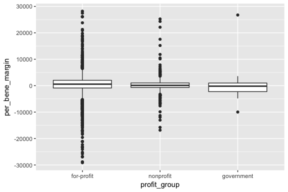
ggplot() +
geom_boxplot(data = graph_data, aes(x = profit_group, y = per_bene_margin))
ggplot() +
  geom_boxplot(data = graph_data, aes(x = profit_group, y = days_per_bene))
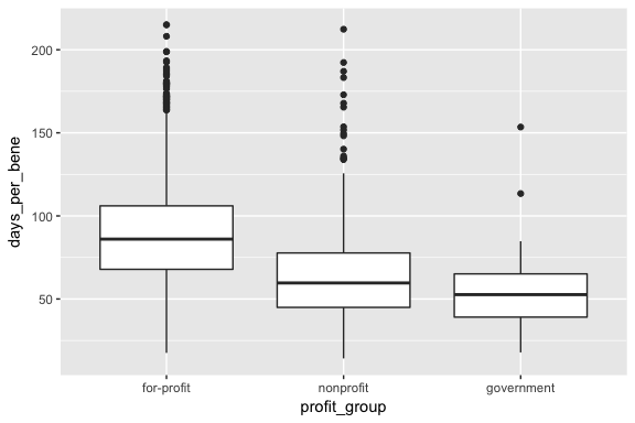
It looks like government-run agencies have very little variance in per-beneficiary profit rates. Overall, it looks like for-profit agencies have higher average profit rates than nonprofit agencies, but the both show high variation. In terms of length of stay, for-profit agencies tend to be higher.
# use the state geometry files from the 'maps' package
state_map = map_data("state")

# make lower, to conform to state_map values
states <- data.frame(state.abb, state.name)
names(states) <- c("state", "state_name")
states$state <- as.character(states$state)
states$state_name <- tolower(states$state_name)

graph_data %<>% full_join(states, by = "state")

mean_by_state <- graph_data %>%
  filter(!is.na(state_name), !is.na(profit_group)) %>%
  group_by(state_name, profit_group) %>%
  summarize(
    mean_margin = mean(per_bene_margin, na.rm = T),
    mean_days = mean(days_per_bene, na.rm = T)
  )

ggplot() +
  geom_map(data = mean_by_state,
           aes(map_id = state_name, fill = mean_margin),
           map = state_map) +
  expand_limits(x = state_map$long, y = state_map$lat) +
  facet_wrap(~profit_group) +
  scale_fill_gradient(low = "white", high = "blue")
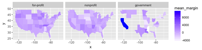
There doesn’t seem to be much of a pattern regarding operating margins, either across regions or across profit status. However, when looking at the average length of stay, we see a clearer trend: for-profit hospices report higher averages than other types, and the effect seems concentrated in the south.
ggplot() +
  geom_map(data = mean_by_state,
           aes(map_id = state_name, fill = mean_days),
           map = state_map) +
  expand_limits(x = state_map$long, y = state_map$lat) +
  facet_wrap(~profit_group) +
  scale_fill_gradient(low = "white", high = "blue")
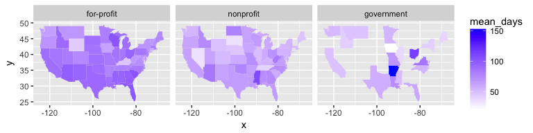
Of course, both our measure of patients and of days are crude. They are aggregates across all payer types (Medicare, Medicaid, other insurance, private pay), and the count of days does not discern between inpatient care and in-home treatment. Additional patterns might appear by taking a finer look at those aspects of the data.
Conclusion
This was just a demonstration with one year’s worth of data from one sector. Hospices also appear in the costs reports for SNF’s, HHA’s, and hospitals. In fact, after extracting data from those sources, the dataset we use at Vanderbilt increases from ~2800 to ~4200 hospices per year. In addition, the data is longitudinal, so there are ample opportunities for exploration of trends.
While I only looked at profit-status and state as levels of aggregation
here, we could repeat the analyses with Dartmouth’s HRR
boundaries.
In addition, the cost reports also have information on self-reported
membership in a healthcare chain, which would add another layer of
granularity to the analysis (note: we have found the chain-related
variables to be much less reliable and requiring of significant checking
and recoding). Finally, since the 6-digit prvdr_num in the cost
reports is frequently used as a unique identifier in other CMS data
sources, the cost report data is easily merged with other datasets. The
Provider of Services
file,
for instance, has yearly information on facility staffing levels.